Fourier Transforms

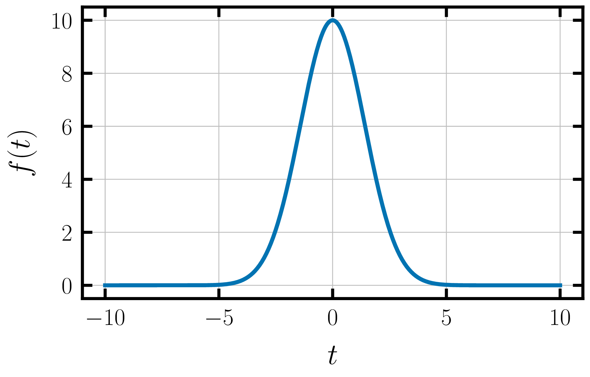
Fourier Series apply only to functions that are periodic or that can be assumed to be periodic. Unfortunately, most of the functions that we encounter in real life are aperiodic in nature. For example, the ubiquitous Gaussian distribution shown in the figure below, is aperiodic in nature and cannot be assumed to be periodic.

Gaussian Distribution

The Fourier transform is a generalization of the Fourier Series to all functions, including aperiodic functions.

$\begin{equation} \begin{split} f(t) &= \frac{1}{2\pi}\int_{-\infty}^{\infty} F(\omega) e^{j\omega t} \; \rm{d}\omega \\[0.4cm] F(\omega) &= \int_{-\infty}^{\infty} f(t) e^{-j\omega t} \; \rm{d}t \end{split} \end{equation}$

Unfortunately, it is a little difficult to have intuition for Fourier transforms. The best way to develop intuition is to familiarize yourself with some common Fourier transform pairs. Hopefully, most of the functions you will encounter later will only be a combinations of these functions.

Common Fourier Transform Pairs

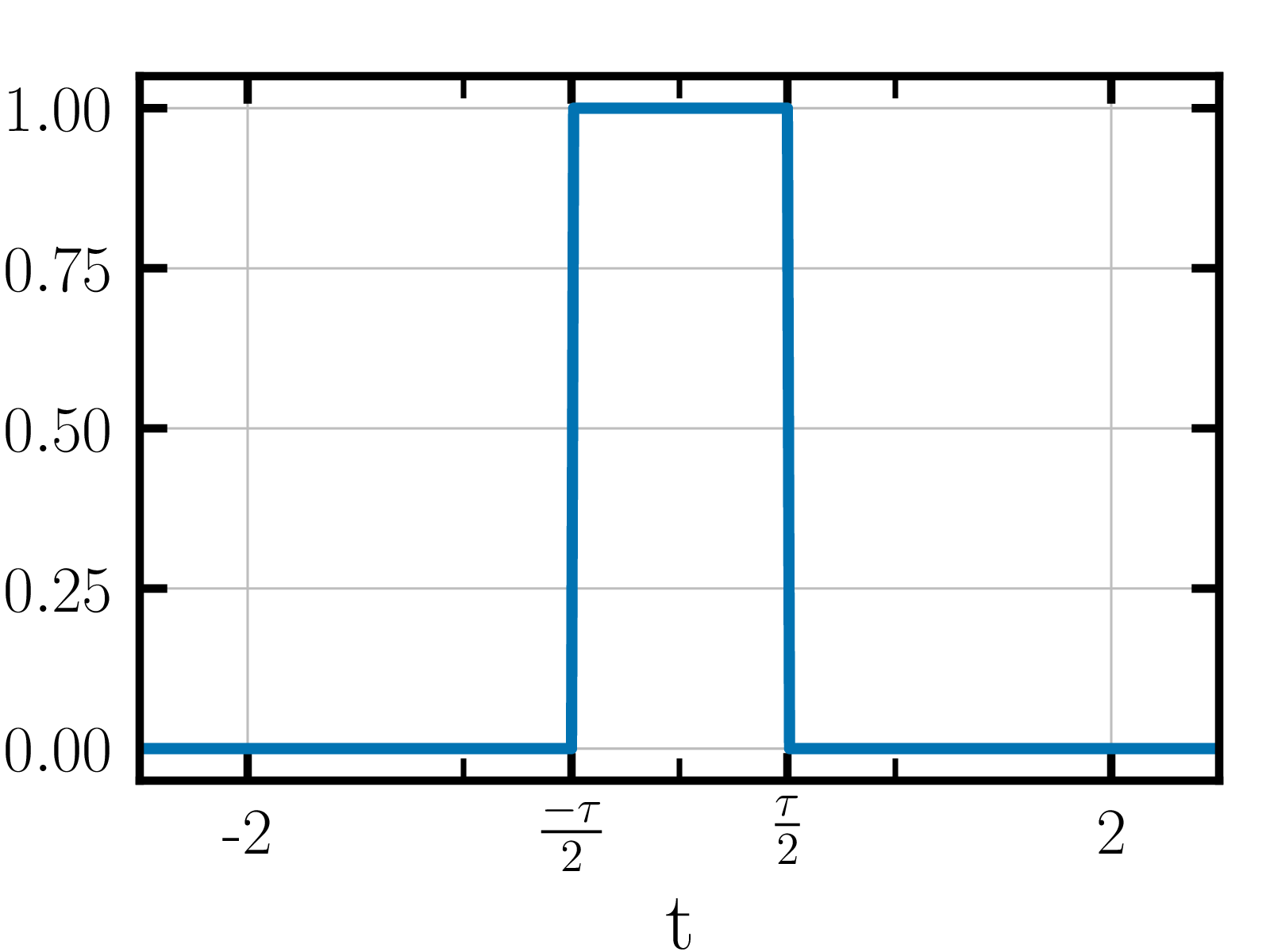
1. Rectangular Function

Also sometimes called the top-hat function. You will come across this function multiple times in digital signal processing and maybe even otherwise. This can be seen as the basic “selector” function, that applies to periodic signals to make them aperiodic.

TopHat

$\text{rect}\left(\frac{t}{\tau}\right) = \begin{cases} 1, & |t|\leq \frac{\tau}{2} \\ 0, & \text{otherwise} \\ \end{cases}$

It is worth deriving the Fourier transform of this function by going through the integral (just for fun).

$\begin{equation*} \begin{aligned} F(\omega) &= \int\limits_{-\tau/2}^{\tau/2} e^{-j\omega t} dt \\[0.3cm] &= \frac{-1}{j\omega} \left[e^{-j\omega t}\right]_{t=-\tau/2}^{t=\tau/2} \\[0.3cm] &= \frac{-\left[e^{-j\omega\tau /2} - e^{j\omega\tau /2}\right]}{j\omega}\\[0.3cm] &= \frac{\left[e^{j\omega\tau /2} - e^{-j\omega\tau /2}\right]}{j\omega} \\[0.3cm] &= \frac{\sin{\left(\frac{\omega\tau}{2}\right)}}{\omega/2} \\[0.3cm] &= \tau \frac{\sin{(\pi \nu \tau)}}{\pi \nu \tau} \\[0.3cm] &= \tau \text{sinc}\left(\frac{\omega\tau}{2}\right) = \tau \text{sinc}(\pi \nu \tau) \\[0.3cm] \end{aligned} \end{equation*}$

The final function, called the sinc-function is an infinite function that is defined at all values of $\omega$. The Fourier transform pair between a top-hat and a sinc-function are shown below:

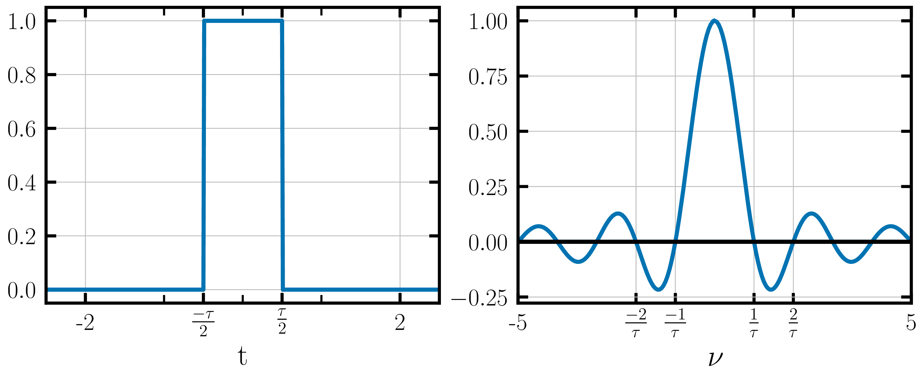
FT top hat — sinc$\left(\frac{\pi t}{\tau}\right)$ $\longleftrightarrow$ $\tau \; $rect($\tau \nu$)

One useful thing about Fourier transform pairs is that they are inter-changable. That is, the Fourier transform of a top-hat function is a sinc-function and the Fourier transform of a sinc-function is top-hat function again.

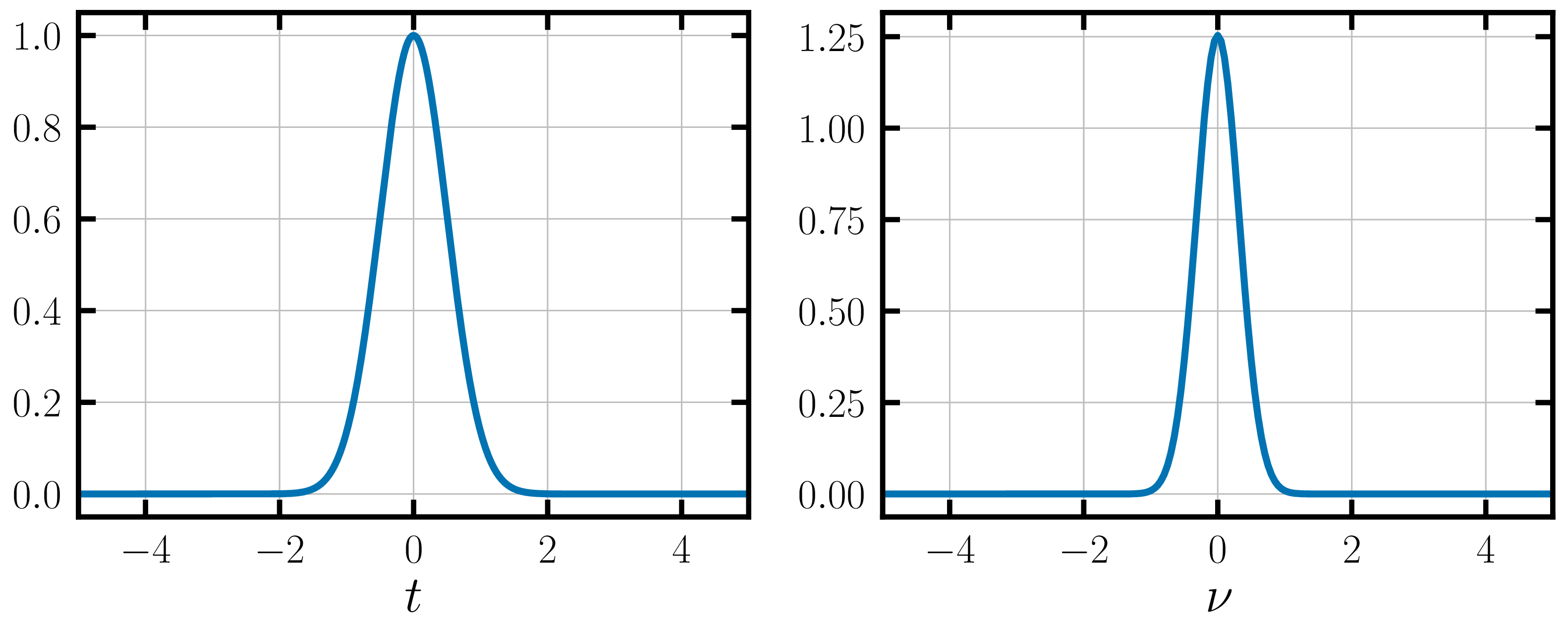
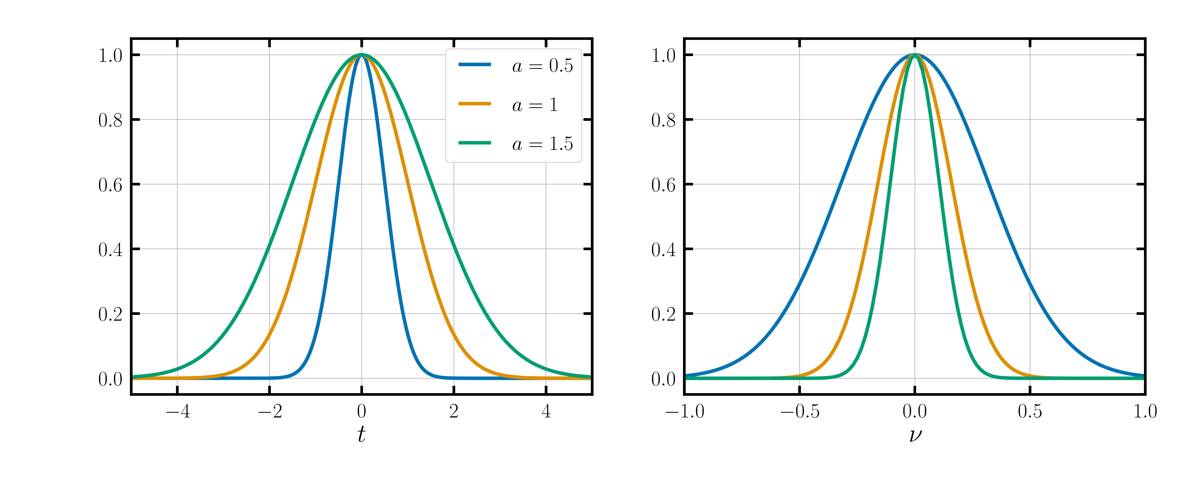
FT sinc — sinc$\left(\frac{\pi t}{\tau}\right)$ $\longleftrightarrow$ $\tau \; $rect $\left(\tau \nu\right)$

2. Gaussian Distribution

This will probably be the easiest to remember since the Fourier transform of a Gaussian function is just another Gaussian function!

However, notice the inverse relationship between the two widths– if the time-domain Gaussian is very fat (large variance), the frequency-domain Gaussian is proportionally thin and vice-versa.

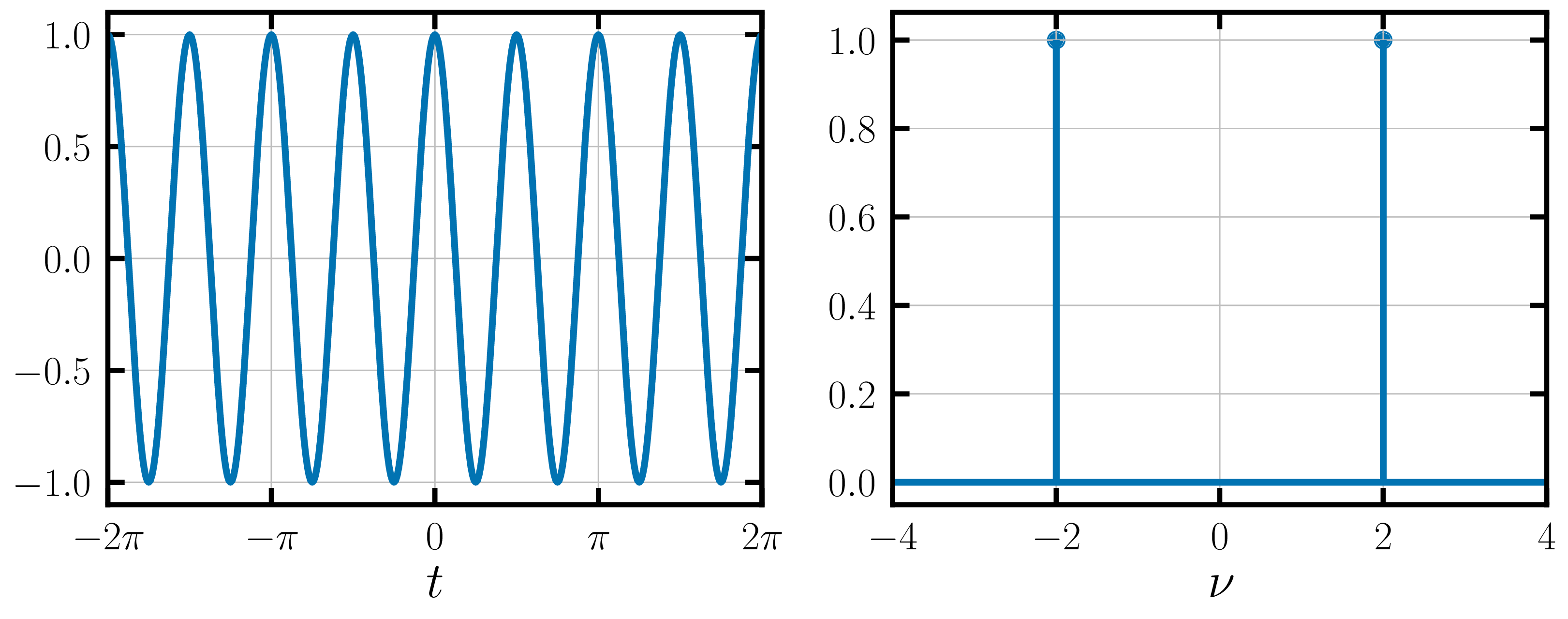
FT Gaussian — $e^{-\frac{t^2}{2a^2}}$ $\longleftrightarrow$ $\sqrt{2\pi}a e^{-2\pi^2 a^2 \nu^2}$

3. Cosine Wave

This is a trick question: What is the Fourier Transform of a periodic function?

Bring out that pen and paper again, we’re going to derive the Fourier Transform of the cosine function with a known frequency $f(t) = \cos{(\omega_0 t)}$.

$\begin{equation*} \begin{aligned} F(\omega) &= \int\limits_{-\infty}^{\infty} \cos{(\omega_0 t) e^{-j\omega t}} dt \\[0.3cm] &= \frac{1}{2} \int\limits_{-\infty}^{\infty} \left[e^{j\omega_0 t} + e^{-j\omega_0 t}\right] e^{-j \omega t} dt \\[0.3cm] &= \frac{1}{2}\int\limits_{-\infty}^{\infty} e^{-j(\omega - \omega_0)t} dt + \frac{1}{2}\int\limits_{-\infty}^{\infty} e^{-j(\omega + \omega_0)t} dt \\[0.3cm] &= \frac{1}{2}\left[\delta(\omega-\omega_0) + \delta(\omega+\omega_0)\right] \end{aligned} \end{equation*}$

The last step introduced a new function $\delta(\omega)$, which is called the Dirac-Delta function. This function is a way for mathematics to tell you that you have encountered a discreet function on your quest for a continuous one.

Dirac-Delta function $\delta(\omega)$ is zero everywhere, expect $\omega=0$.

Even though we acted dumb and tried to Fourier transform a function which should be decomposed into a Fourier series, mathematics returned us a function that is non-zero exactly at the frequency of our original cosine wave.

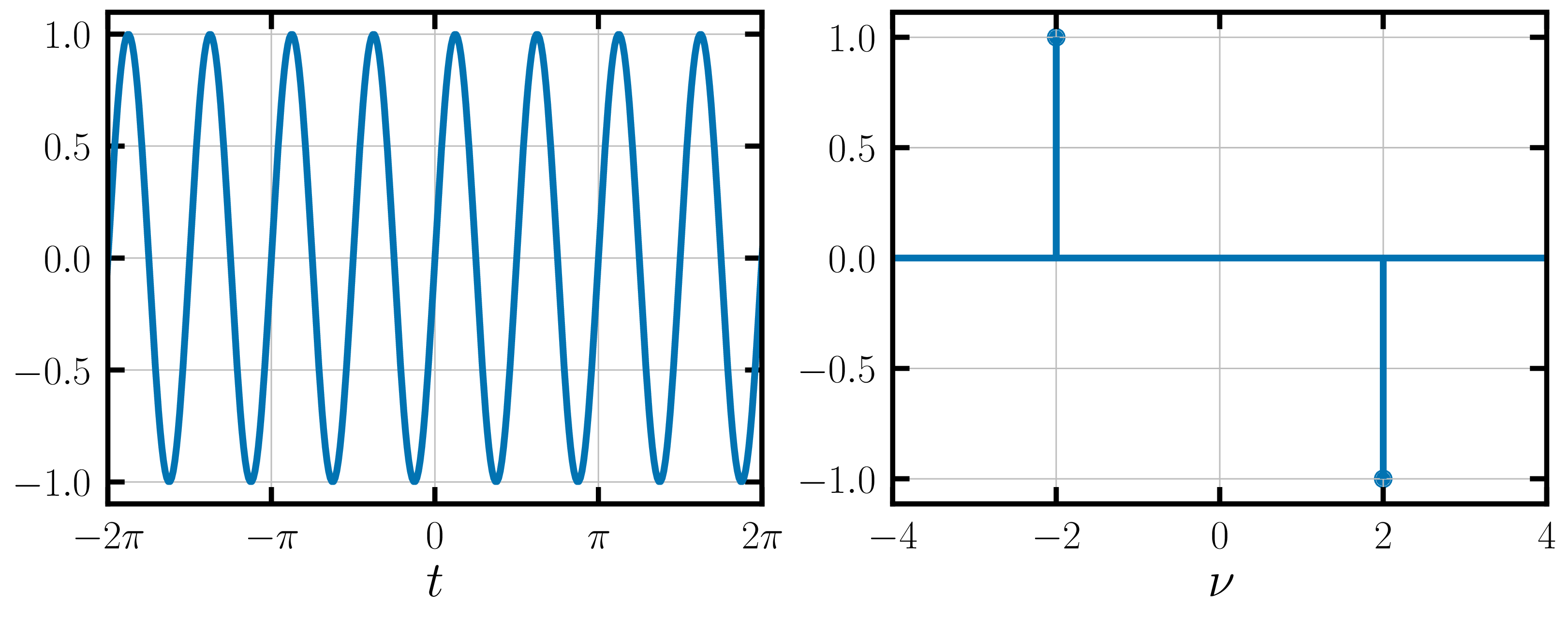
FT Cosine — $\cos{(2\pi \nu_0 t)}$ $\longleftrightarrow$ $\left[\delta(\nu + \nu_0) + \delta(\nu - \nu_0)\right]$

4. Sine Wave

This derivation is exactly analogous to the one we did for a cosine wave.

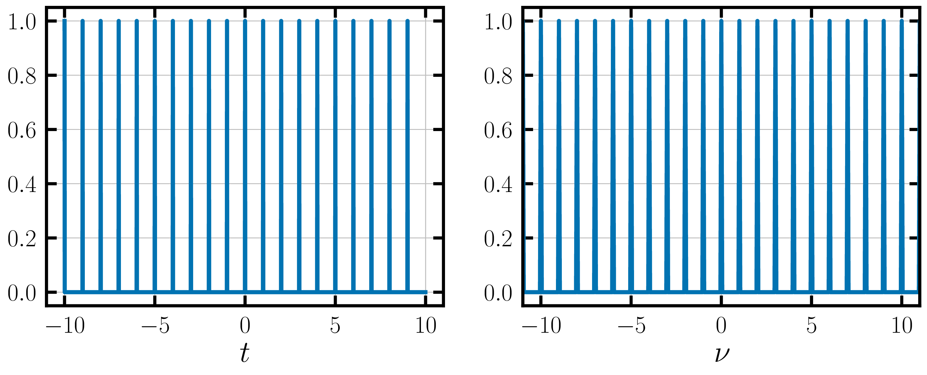
FT Sine — $\sin{(2\pi \nu_0 t)}$ $\longleftrightarrow$ $j\left[\delta(\nu + \nu_0) - \delta(\nu - \nu_0)\right]$

5. Dirac Comb

A Dirac Comb is a series of Dirac-Delta functions that are seperated by some known time-period $t_0$ (Equation 5). This will be an extremely useful function when we are sampling analog signals for digitizing them.

$\begin{equation} f(t) = \sum\limits_{k=-\infty}^{\infty} \delta(t-kt_0) \end{equation}$

The Fourier transform of a Dirac comb is another Dirac comb. Much like the Gaussian, the time period of the comb in time-domain has an inverse relationship with the fundamental frequency of the comb in the frequency-domain. That is, the “finer” the comb in time-domain, the “coarser” the Fourier transform comb.

FT Dirac Comb — $\sum\limits_{k=-\infty}^{\infty} \delta(t-kt_0)$ $\longleftrightarrow$ $\sum\limits_{m=-\infty}^{\infty}\delta\left(\nu - \frac{m}{t_0}\right)$

Summary: Fourier Transform Pairs

	$f(t)$	$F(\nu)$
Top Hat	rect($\frac{t}{\tau}$)	sinc($\pi \nu \tau$)
Gaussian	$e^{-\frac{t^2}{2a^2}}$	$e^{-2\pi^2 a^2 \nu^2}$
Cosine	$\cos{(2\pi \nu_0 t)}$	$\left[\delta(\nu + \nu_0) + \delta(\nu - \nu_0)\right]$
Sine	$\sin{(2\pi \nu_0 t)}$	$j\left[\delta(\nu + \nu_0) - \delta(\nu - \nu_0)\right]$
Delta Train	$\sum\limits_{k=-\infty}^{\infty} \delta(t-kt_0)$	$\sum\limits_{m=-\infty}^{\infty}\delta\left(\nu - \frac{m}{t_0}\right)$

Properties of Fourier Transforms

1. Linearity

$\begin{equation*} \begin{split} af(t) &\longleftrightarrow aF(\omega) \\[0.3cm] af(t) + bg(t) &\longleftrightarrow aF(\omega) + bG(\omega) \\ \end{split} \end{equation*}$

2. Scaling

$\begin{equation*} f(at) \longleftrightarrow \frac{1}{|a|} F\left(\frac{\omega}{a}\right) \end{equation*}$

FTP Scaling

3. Shift

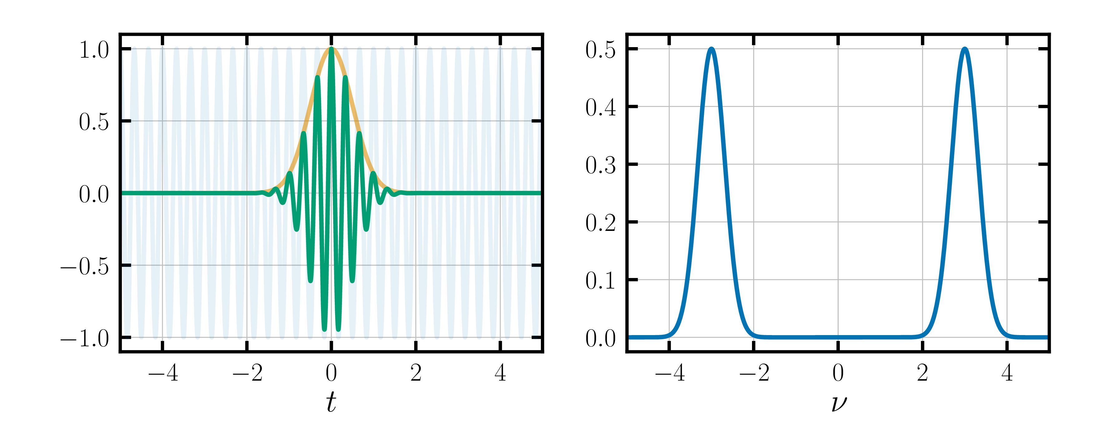
$\begin{equation*} \begin{split} f(t-t_0) &\longleftrightarrow e^{-j\omega t_0} F(\omega) \\[0.3cm] f(t) e^{j\omega_0 t} &\longleftrightarrow F(\omega-\omega_0) \end{split} \end{equation*}$

In radio transmission, you might have heard of FM radio channels. The FM stands for ‘Frequency Modulation’ which uses the shift property of Fourier transforms to change the transmission frequency of the base audio signal. Say you want to transmit a Gaussian wave centered at zero, but you can only transmit at a higher frequency. By multiplying the original signal with a cosine wave at the transmission frequency, you can up-convert the original Gaussian.

4. Symmetry

Analogous to the rule in Fourier Series, even and odd functions have characteristic signatures in their Fourier transforms.

$\begin{equation} \begin{split} f(t) \text{ real and even } &\longleftrightarrow F(\omega) \text{ real and even} \\ f(t) \text{ real and odd } &\longleftrightarrow F(\omega) \text{ imaginary and odd} \end{split} \end{equation}$

A cosine wave is an even function, and a sine wave is an odd function. Look at their Fourier transforms for a demonstration of this property.

5. Derivative and Integration

These are slightly esoteric properties that you might face in advance digital signal processing techniques. You might encounter it in physics or control systems more often.

$\begin{equation*} \frac{d^nf}{dx^n} \longleftrightarrow (j\omega)^n F(\omega) \end{equation*}$ $\begin{equation*} \int\limits_{-\infty}^{t} f(\tau) d\tau = \frac{1}{j\omega} F(\omega) + \pi F(0)\delta(\omega) \end{equation*}$

6. Convolution Theorem

This is probably the most important application of Fourier transforms. Convolution is a mathematical operation (like multiplication or addition) that operates on two functions– say, $f(t)$ and $g(t)$. It is mathematically defined as follows:

$\begin{equation*} f(t) * g(t) = \int\limits_{-\infty}^{\infty} f(\tau) g(t-\tau) \; d\tau \end{equation*}$

You will learn about the applications of convolution if you are doing any course from probability to natural language processing, and very often in electronics or electrical engineering or radio astronomy.

I will not explain convolution very much here (the wikipedia page on it has a pretty good introduction), except point out that it is not simply multiplying the two functions.The figure below shows the product of the two functions $f(t)$ and $g(t)$ and their convolution.

convolution_1

convolution_2

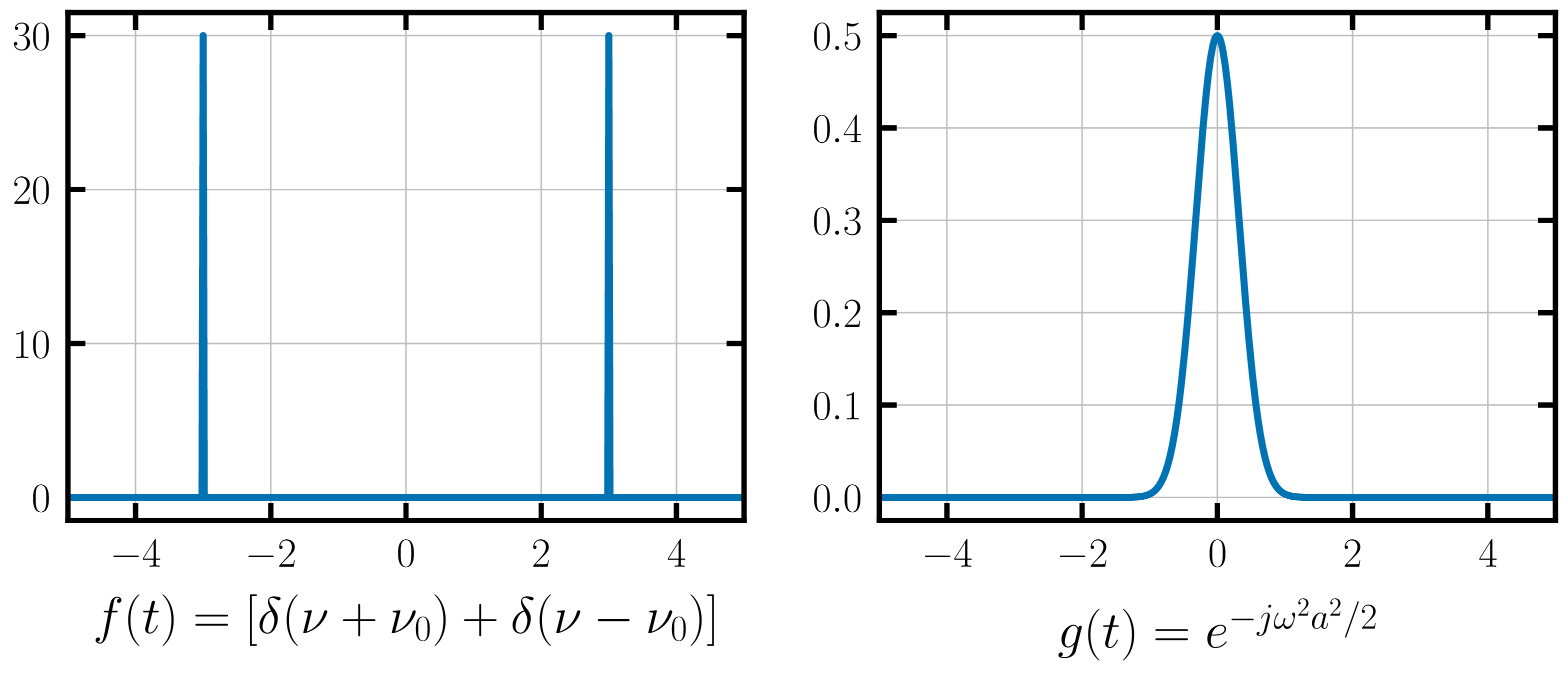
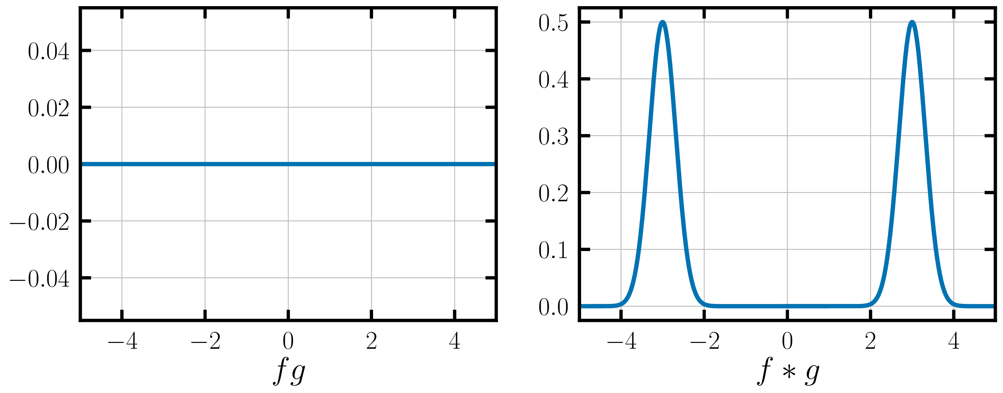
The convolution of two functions in the time domain translates to their product in the frequency-domain, and vice-versa. This is shown by the equations below:

$\begin{align*} f(t) * g(t) &\longleftrightarrow F(\omega)G(\omega) \\[0.5em] f(t)g(t) &\longleftrightarrow F(\omega) * G(\omega) \end{align*}$

The convolution theorem, as the above equations are called, is important because it simplifies the $O(N^2)$ convolution operation to the gentler $O(N\log{N})$ fourier transform operation for digital signals. This decrease in algorithm complexity is entirely due to the Fast Fourier Transform (FFT) algorithm by Cooley and Tukey (1965) which we will talk about in the Discreet Fourier Transform section.

Spectral Leakage

An interesting combination of all the facts we have learned so far is spectral leakage. Let me explain it through an example:

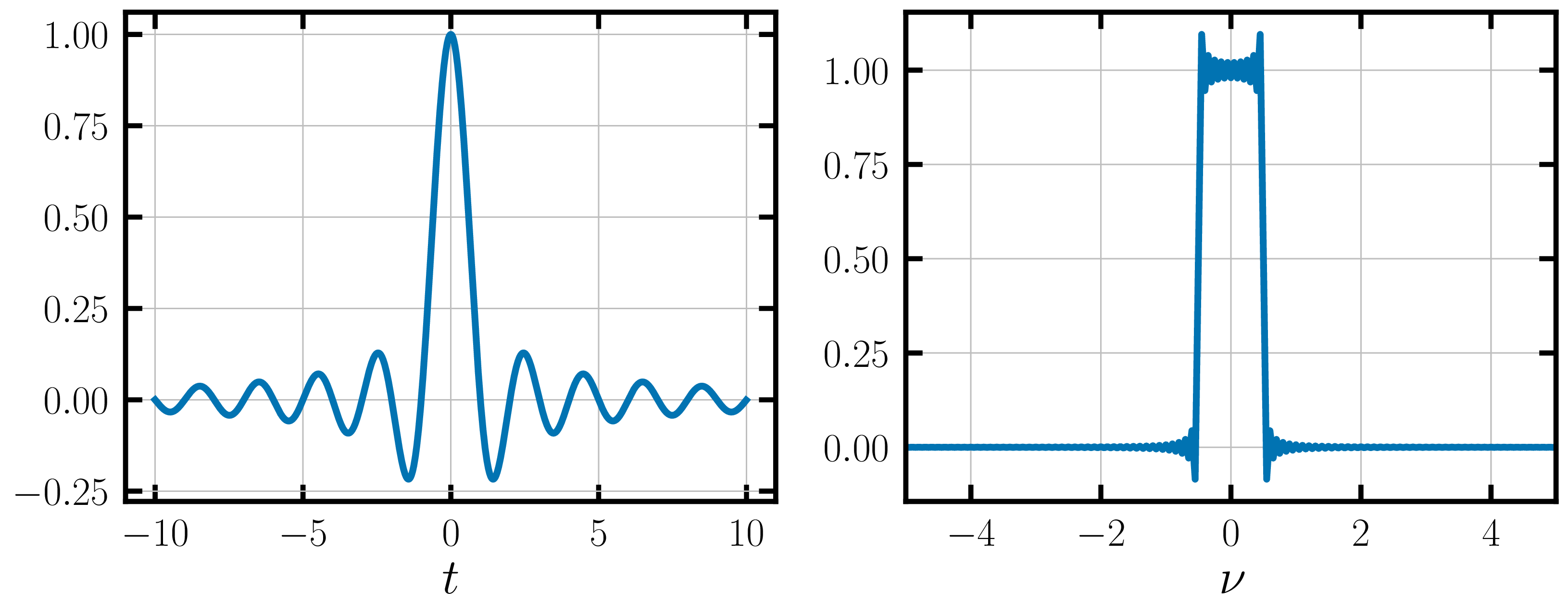
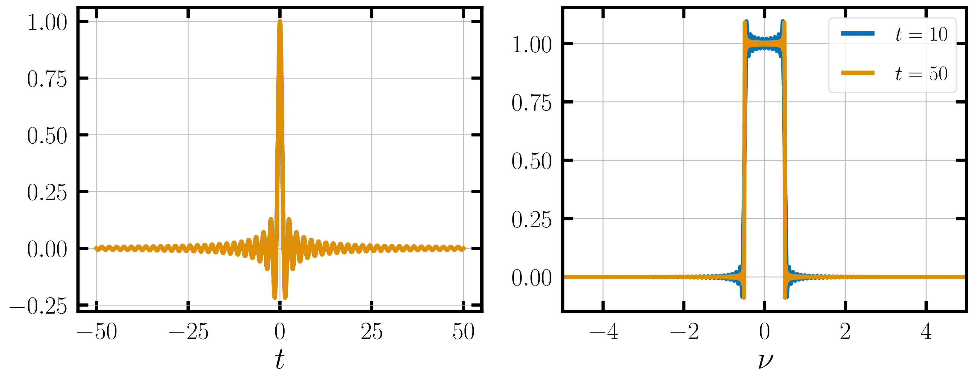
Say, you want to compute the Fourier transform of a sinc-function on a computer. The sinc-function is an infinite signal that extends from negative infinity to infinity. Unfortunately, computers cannot deal with infinite signals and you will need to truncate the sinc-function at some point for encoding it on a computer. This is equivalent to multiplying the sinc-function with a top-hat function with a width equal to the length of the sinc-function you are encoding.

The Fourier transform of the product of two functions in the time-domain is equal to the convolution of their individual Fourier transforms, according to the convolution theorem. Hence, the function that the computer generates by Fourier transforming the truncated sinc-function, is a convolution of the top-hat function that we should really obtain with a another sinc-function!

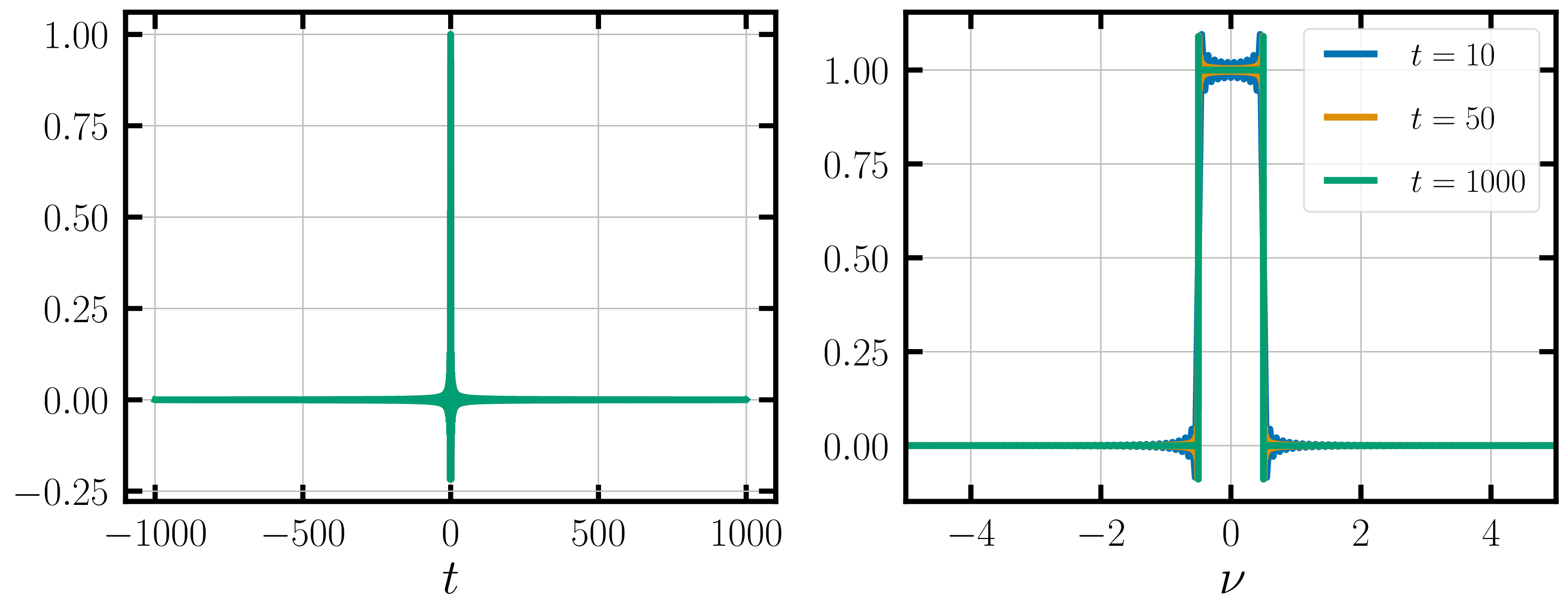
The scaling property that we discussed before is important here. If the top-hat function that is truncating the sinc-function in the time-domain is wide, the corresponding sinc-function that convolves the result in the frequency-domain will be narrow. That is, the longer the sinc-function we consider in the time-domain, the sharper the frequency domain signal will be. This is illustrated in the plots below.

This effect of not obtaining the “complete” Fourier transform of a digitized, truncated signal is called Spectral Leakage. This effect can be minimized by considering a longer-window of the time-domain signal but cannot be completely eliminated for infinite signals.

spectral_leakage_1

spectral_leakage_2

spectral_leakage_3

Summary: Properties of Fourier Transforms

Linearity	$af(t) \longleftrightarrow aF(\omega)$
Scaling	$f(at) \longleftrightarrow \frac{1}{\|a\|}F\left(\frac{\omega}{a}\right) $
Time Shift	$f(t-t_0) \longleftrightarrow e^{-j\omega t_0} F(\omega)$
Frequency Shift	$f(t)e^{j\omega_0 t} \longleftrightarrow F(\omega - \omega_0)$
Derivative	$\frac{d^nf}{dx^n} \longleftrightarrow (j\omega)^n F(\omega)$
Convolution	$f(t) * g(t) \longleftrightarrow F(\omega)G(\omega)$
Correlation	$f(t) \star g(t) \longleftrightarrow F(\omega)G^*(\omega)$

Deepthi Gorthi Radio astronomer