Deepthi Gorthi Radio astronomer
Projects
Fast Fourier Transform Correlators
![]() January 2018 - Present
January 2018 - Present
A correlator is the signal processing pipeline that forms the backend of any array of radio antennas built for astronomy. In a radio interferometer, an image of the sky is reconstructed from cross-products of antenna voltages called visibilities. A correlator computes these visibilities for every frequency channel in the bandwidth of the radio antenna.
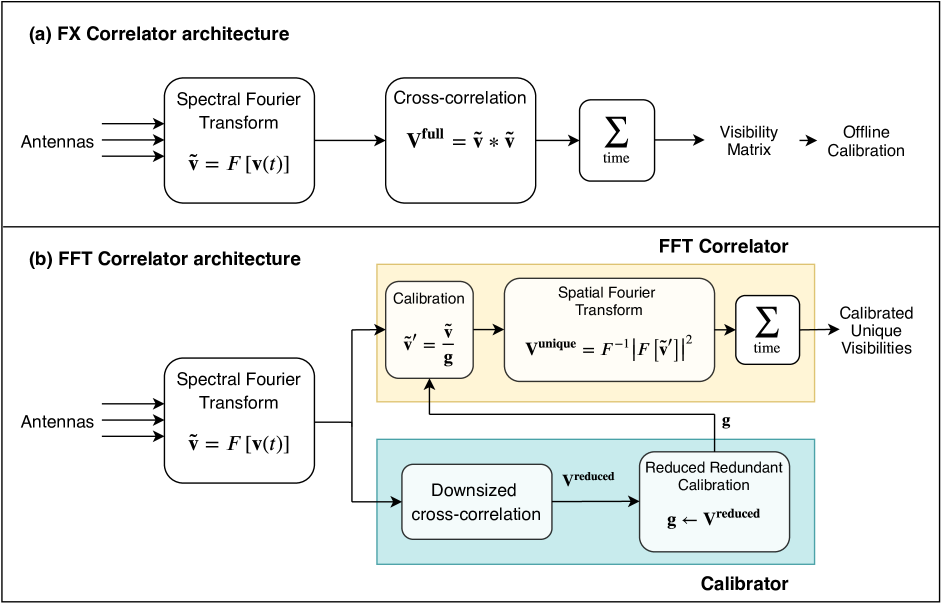
Traditionally, radio interferometers from the Very Large Array (VLA) to the Atacama Large Millimetre Array (ALMA), have had a correlator architecture that is close to the one shown in Panel (a) of the above figure. A spectral Fourier transform first converts the time-domain voltages into a spectrum with narrow frequency channels. In the second stage, a cross-correlation computes the visibility matrix ${\bf V^{full}}$ by multiplying the signal from every antenna with the signal from every other antenna in the array. This cross-correlation operation requires $O(N_a^2)$ computational resources if $N_a$ is the number of antennas in the array.
Recently, there has been a rebirth of interest in low-frequency radio astronomy application that require $N_a\gg 1000$ antennas where such traditional correlator architectures could be non-viable due to the high computational costs. In 2010, MIT professors Max Tegmark and Matias Zalarriaga revived another way of computing these cross-correlations which I call an FFT-Correlator. This architecture (with my own modifications) is shown in Panel (b) of the above figure. In an FFT-Correlator, the visibility matrix ${\bf V^{unique}}$ is computed through a spatial Fourier transform of the signal from all the antennas in the array. Leveraging the Cooley-Tukey Fast Fourier Transform algorithm, the computational cost of such a correlator will only scale as $O(N_a\log_2N_a)$ making it affordable to build large antenna arrays.
There are two main caveats to such a correlator: (a) it only operates on antennas that are on a regular grid, like phased arrays and (b) it averages the cross-products of antenna-pairs that are equidistant from each other. The former creates an interferometer design restriction that is satified for the class of interferometers that target the 21 cm cosmological signal. More recently, interferometers with antennas on a regular grid are being proposed for FRB and Pulsar science as well. The latter poses a real problem because visibilities of antenna-pairs that are equidistant are dissimilar unless calibrated. The averaging in the FFT-correlator can lead to loss of signal that prevents post-processing calibration.
Algorithms that are capable of calibrating antennas operate on visibilities, not voltages. However, the spatial Fourier transform that computes these visibilities cannot do so unless the antenna voltages are calibrated. For my Ph.D. thesis, I worked on two calibration schemes that require only $O(N_a\log_2N_a)$ computational resources for calibrating the antenna voltages. A smaller visibility matrix ${\bf V^{reduced}}$ is constructed for the purpose of computing per-antenna calibration parameters. This calibration architecture is shown within the blue box in the figure above.
The two calibration schemes, that are modifications of redundant-baseline calibration, can be implemented within the calibrator:
-
Low-cadence calibration ($\texttt{lowcadcal}$): The antenna-pairs are cross-correlated in a round-robin fashion using $O(N_a\log_2N_a)$ computational resources, till the full visibility matrix is constructed. This matrix is then used for redundant-baseline calibration.
-
Subset redundant calibration ($\texttt{subredcal}$): Only a limited set of antenna-pairs are cross-correlated using $O(N_a\log_2N_a)$ computational resources. This truncated visibility matrix is used for redundant-baseline claibration.
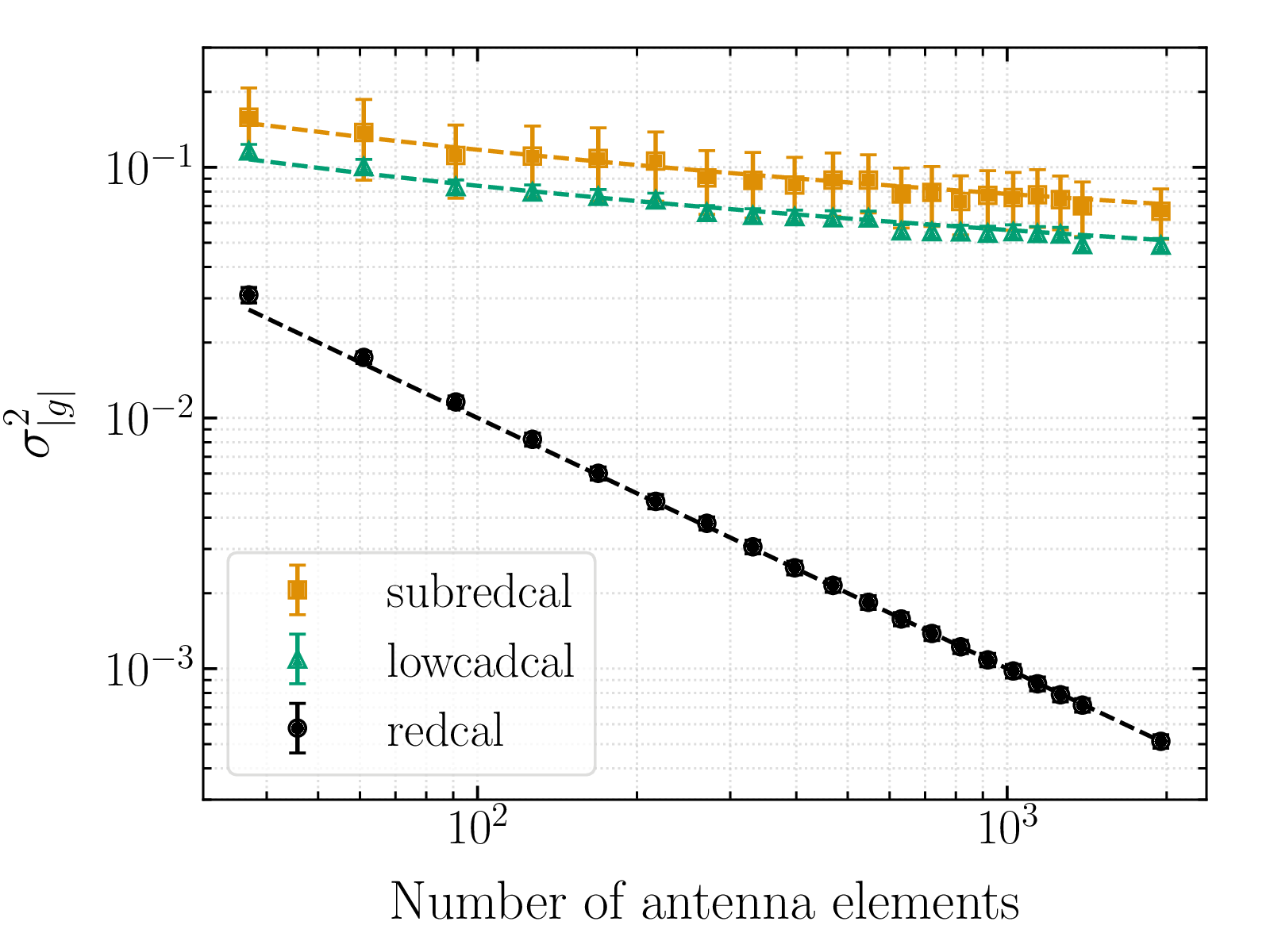
The variance in the antenna gains computed using low-cadence calibration and subset redundant calibration, when compared to regular redundant-baseline calibration ($\texttt{redcal}$) are shown above for various array sizes. Both the modified calibration schemes have a $\left(1/\log_2N_a\right)$ scaling in gain variance (shown by the dashed lines) while redundant-baseline calibration has a $\left(1/N_a\right)$ scaling. While this makes it seem like regular redundant-baseline calibration is the best calibration scheme, it is non-viable for large arrays because of the $O(N_a^2)$ computational cost involved in computing the full visibility matrix. Moreover, the extra precision obtained from redundant-baseline calibration is unnecessary because the final scatter in post-calibrated visibilities is domainted by thermal noise and gain variance only has a negligibly small contribution.
If you want to read about this project in detail, here is a link to my publication.
Correlator for the HERA Interferometer
![]() June 2016 - Present
June 2016 - Present
The Hydrogen Epoch of Reionization Array (HERA) is a radio interferometer that is under construction in the South African Karoo desert. Its science goal is to measure the power spectrum of neutral hydrogen during the Epoch of Reionization (EoR). The power spectrum, much like a radio image, is built from cross-products of antenna voltages called visibilities. These cross-products can also be integrated in time for upto ~10 seconds for HERA-like antennas. Since voltages cannot be integrated in a similar manner, it is advantageous to compute these cross-products in real-time to reduce the storage capacity required.
Astronomers, in general, like to measure power as a function of frequency. The power in each spectral bin holds more information about the source than bolometric power. For instance, in the case of HERA the power as a function of frequency can give us information about the evolution of neutral hydrogen in time. Hence, the backend signal processing pipeline of many radio telescopes consists of a polyphase filterbank (simply, an effective spectral Fourier transform) that can channelize the time-domain data.
The channelizing of antenna voltages and cross-correlation can be performed in any order for a radio telescope. For HERA, we chose to implement the FX-correlator design where the F-engine first computes the spectrum for each antenna and then the X-engine computes the cross-correlation product between every pair of antennas in the array, within each narrow frequency bin.
F-Engine
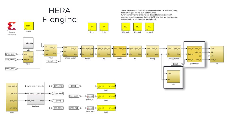
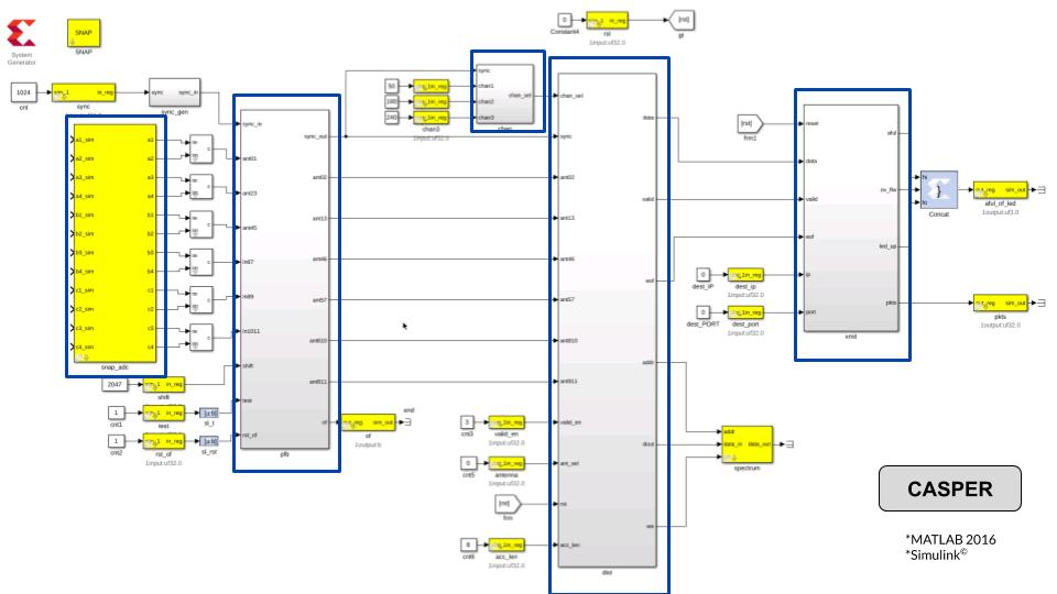
The HERA F-engine was built using CASPER tools on the Kintex 7 XC7K160T Xilinx© FPGA which is part of the SNAP board. The board also contains twelve 8bit, 250 Msps ADCs and two 10Gbps ethernet ports amongst other clocking and GPIO devices.
The ADCs are used in a demux mode where two ADCs are used to sample the voltages from one antenna (one polarization) at 500Msps, to account for the 200MHz bandwidth. A polyphase filterbank then channelizes the data into 4096 spectral bins. This data is packetized into UDP packets and sent to 16 different servers for the next step of cross-correlation. In addition to these basic functions, the HERA F-engine also implements fringe rotation and phase switching(§ 7.5 and 7.7 in Thompson, Moran and Swenson).
My contribution to the F-engine is in many scattered parts. I designed and implemented the $\texttt{corr}$ block (highlighted in the figure above) which computes the cross product of any two inputs on that board. This is useful both as a debugging tool and for monitoring the RFI on site. The autocorrelations computed by the X-engine are integrated for 10 seconds, damping short high-power RFI spikes. The on-board correlator integrates only for 1 second, overcoming this problem. Moreover, since the imaginary bits of autocorrelations are zero by definition, this memory space is allocated to holding the maximum value of autocorrelations for the same 1 second period.
For flexibility in implementation, numerous blocks including the test vector generator $\texttt{eqtvg}$ and $\texttt{packetizer}$ contain programmable BRAMs that need to be set in software. I contributed to the Python scripts that write bit-vectors to these BRAMs and wrote test scripts to verify speed of performance and functionality. The python scripts and the MATLAB Simulink file to this design are available on Github. I also tested, debugged and polished the design and scripts to bring them to a deployable stage. This FPGA design and associated software is currently running on ~64 SNAP boards on site and is expected to expand to 120 boards by December 2020.
X-engine
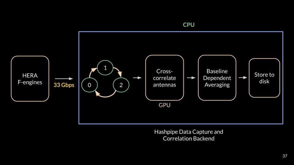
The HERA X-engine is built on 32 Nvidia© GTX-1080 GPU cards, distributed across 16 servers. Each server processes 256 frequency channels and runs two pipelines in parallel, to process the even and odd time samples independently. The net datarate sent to each server, from all the SNAP boards, is ~33Gbps. The pipeline running on each server is based on Hashpipe developed by David Macmahon.
The data is time-multiplexed between two Ethernet ports. The pipeline running on each Ethernet port recieves the UDP packets using packet sockets and puts them into a shared ring buffer. This data is then prepped and transfer to the GPU for cross-correlation. To keep the datarate within the I/O limits of commercial GPUs, the cross-correlation products are integrated in the GPU. The science goals of HERA allows an integration time ~10 seconds and this is used across all baseline-types.
A constant integration time of ~10 seconds across all baselines still produces a large datarate, making both file writing and storage expensive. One way to address this, without compromising on the number of spectral bins, is to average the short baselines for a longer time. The short baselines have a larger synthesized beam allowing longer integration times. Moreover, HERA has more short baselines than long baselines. Between January and October in 2019, I worked on incorporating baseline dependent averaging into the cross-correlation pipeline. The entire X-engine codebase, in C and bash scripts, is available on Github. The final product of this pipeline is HDF5-based files.
Voltage Recorder for Radio Antennas
For the purpose of understanding and verifying the opertion of FFT-Correlators, I built a direct voltage recorder that collects and stores voltage data from radio antennas. Only 0.15% of the spectral bandwidth is stored to disk to keep the end-to-end system implementable on one small server with 12TB storage space.
SNAP-based design
The voltage recorder was implemented using CASPER tools on the Kintex 7 XC7K160T Xilinx© FPGA which is part of the SNAP board. The board also contains twelve 8bit, 250 Msps ADCs and two 10Gbps ethernet ports amongst other clocking and GPIO devices. The Simulink design accounts for all 12 ADC inputs of the SNAP board (each running at <250 Msps) and stores data from three user-selected spectral channels after a 512-point FFT.
For my experiment, I used the Donald C. Backer Precision Array for Probing the Epoch of Reionization (PAPER) antennas to collect direct voltage data. These antennas have a bandwidth of 100 MHz, allowing a single SNAP board to support 12 antennas with one polarization or 6 dual-polarization antennas.
The entire pipeline, from the Simulink design to the software pipeline that can write files is available on Github. Please contact me if you wish to use these files for your project. They are open-source but may not be well-documented enough.