Deepthi Gorthi Radio astronomer
Discrete Time Fourier Transform
The Discrete Time Fourier Transform (DTFT) is a Fourier transform of the sampled, analog function. In all the sections so far, we have only dealt with continuous time-domain signals. If the time-domain signal is discrete (or digitized), the mathematical formulation we need is the DTFT given below:
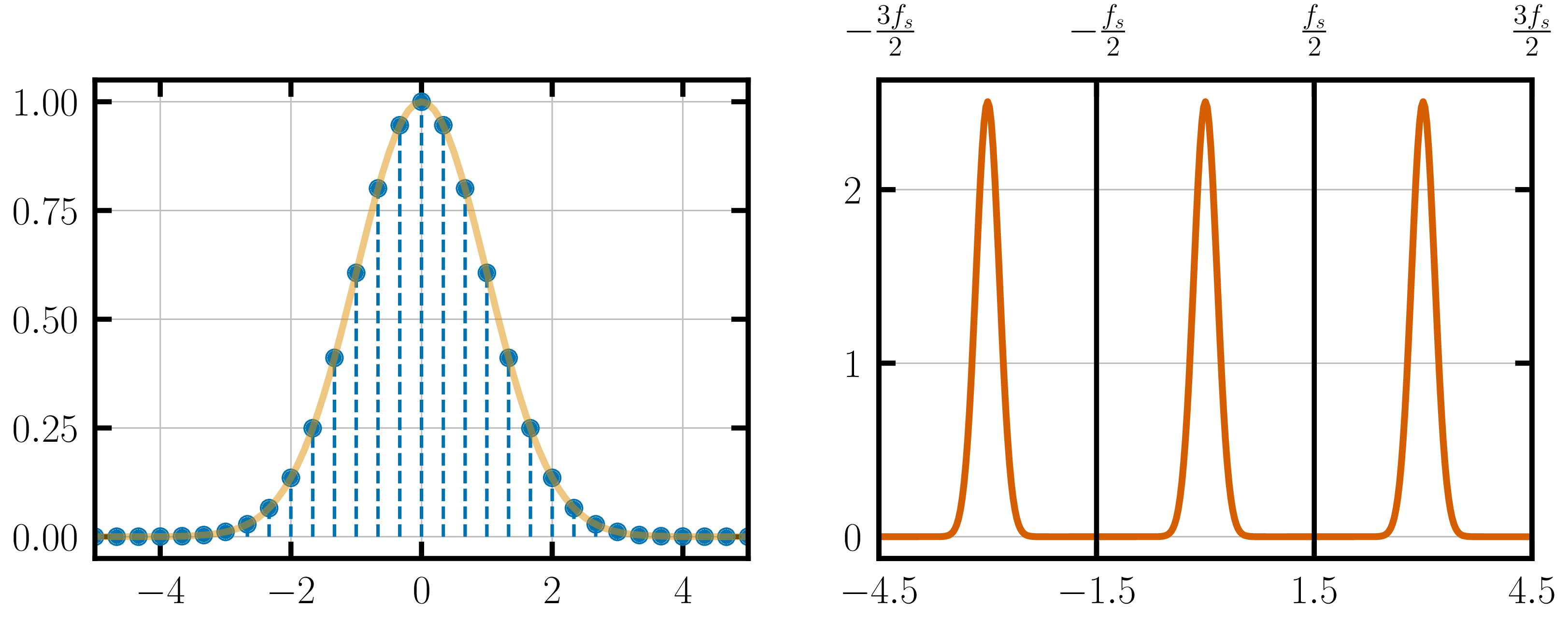
Applying this equation on our over-sampled sine-wave from the previous section:
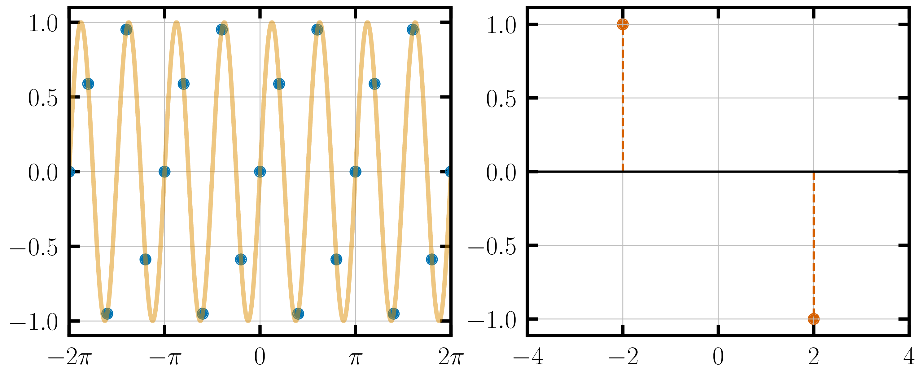
We seem to have obtained exactly the right Fourier transform of the sine-wave!! However, that is not the end of the story. Zooming out on the frequency domain a little more, we find that the original Fourier transform has been repeated across multiple frequencies.
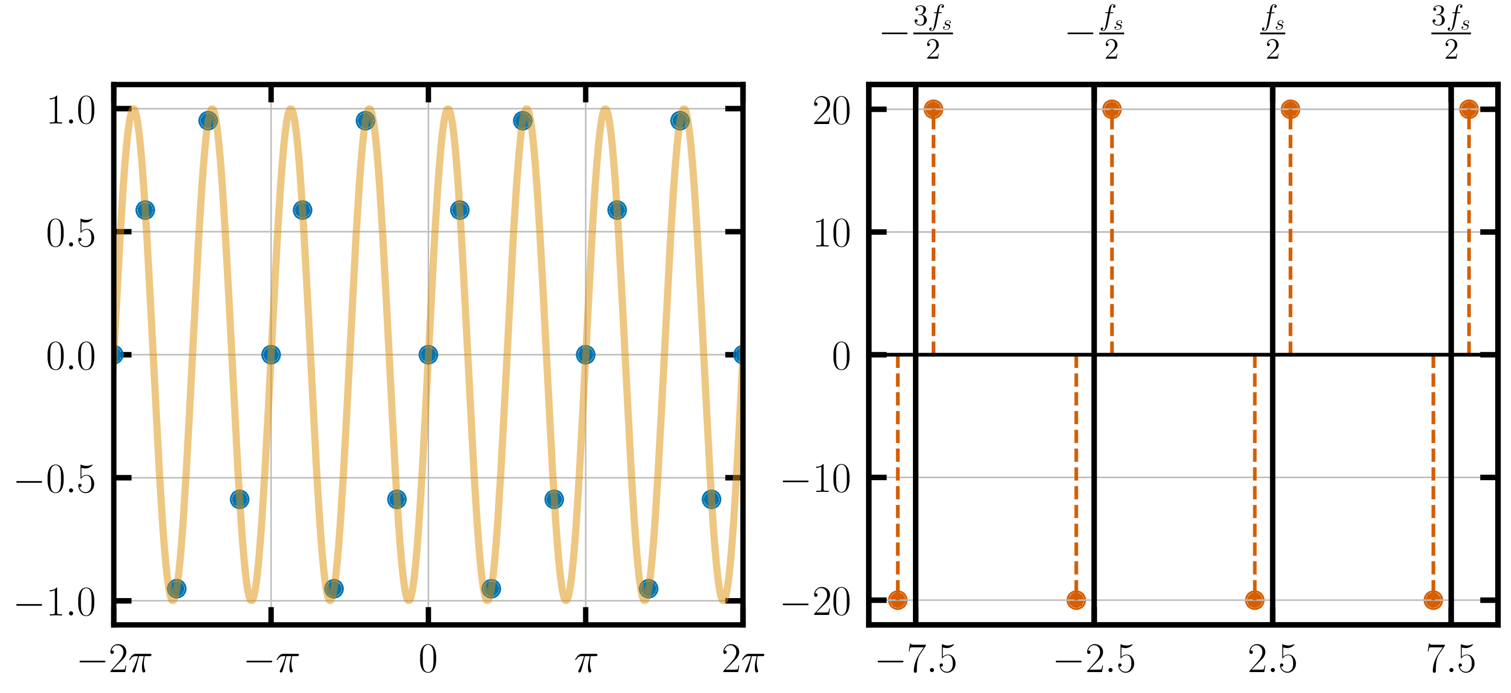
The frequency-domain contains the original Fourier transform at the right frequency and, in addition, also has duplicates of the original FT centered around $f_s$, $2f_s$, $\dots$ and their corresponding negative frequencies.
When you sample an analog signal in the time-domain and compute its Fourier transform, you obtain the Fourier transform of the original analog signal in the frequency range $\left(-\frac{f_s}{2}, \frac{f_s}{2}\right)$.
Outside this frequency range you will find copies of the FT of the original analog signal, centered around $f_s$, $2f_s$, $3f_s$, $\dots$
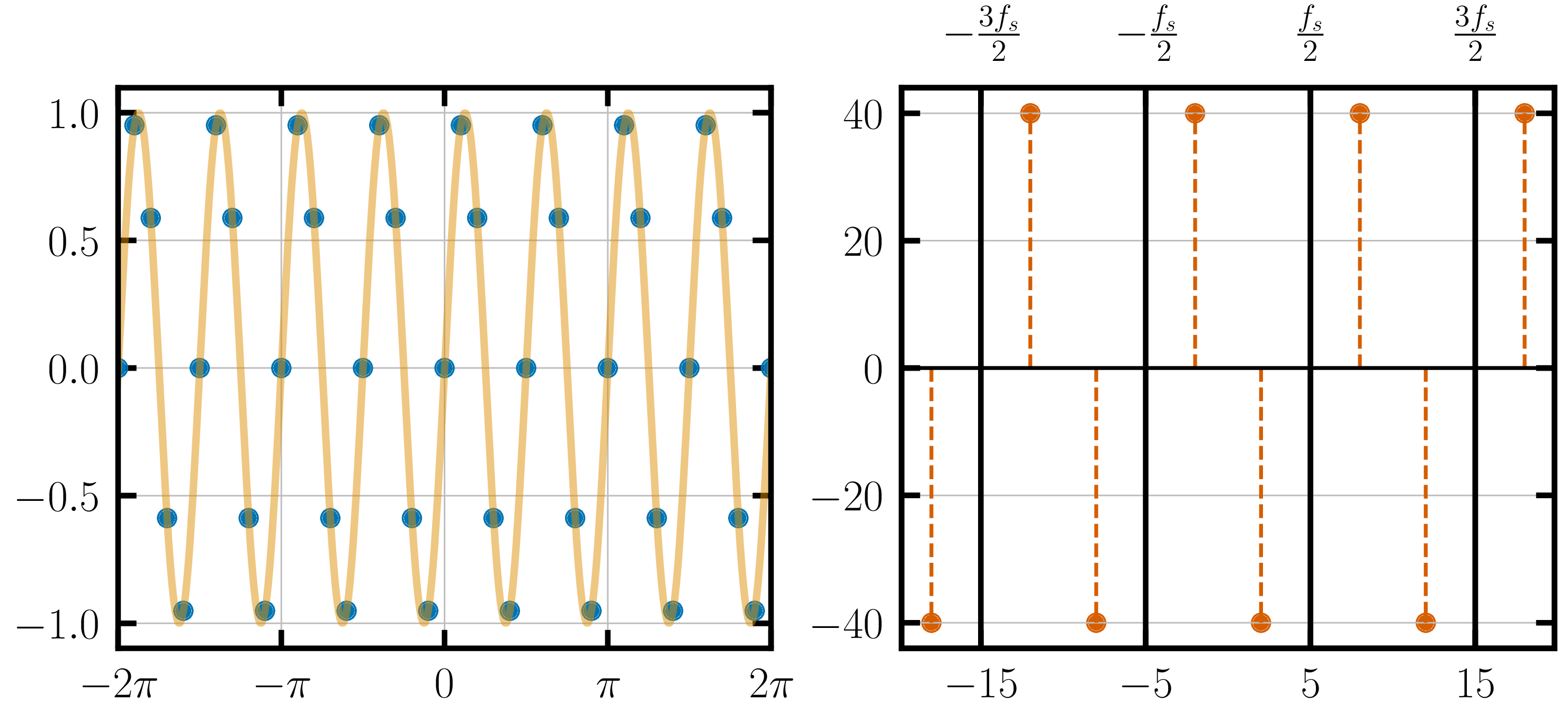
That is essentially the crux of the discreet time Fourier transform. Read it once more to assimilate it. Sampling in the time-domain, creates infinite copies of the frequency-domain centered around multiples of the sampling frequency.
When you sample at a higher frequency, the replicas in the frequency-domain are pushed further away.
What happens when you sample an aperiodic function?
If the FT of the aperiodic function is not infinite, i.e. the Fourier transform of the signal is band-limited or exists within a finite frequency range, the FT can be recovered within the frequency range $\left(-\frac{f_s}{2}, \frac{f_s}{2}\right)$.
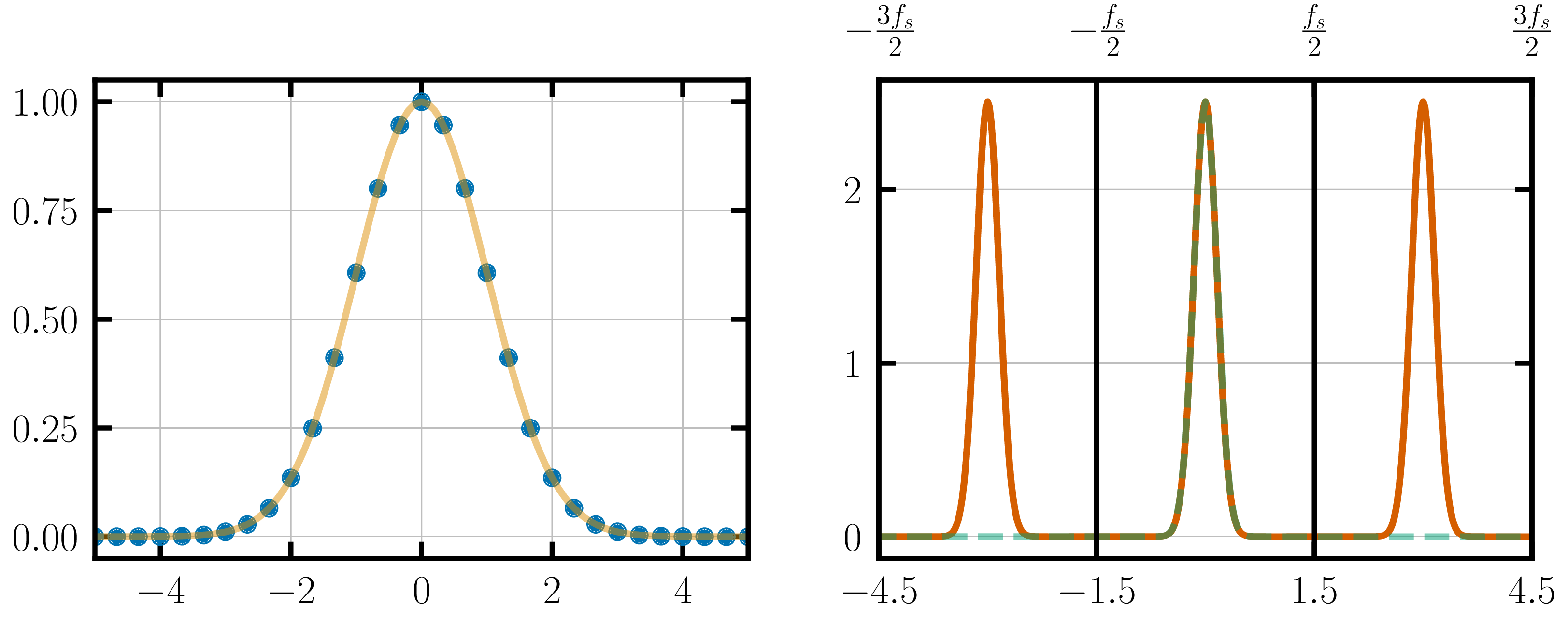
The green-dashed line in the above figure shows the FT of the continuous analog signal while the orange line shows the FT of the sampled discrete Gaussian.
Discrete Time Fourier transform can be seen as multiplying the time-domain signal by a Dirac-comb. The comb has a time-period equal to the inverse of the sampling frequency. According to the convolution theorem, multiplication in the time-domain is equivalent to a convolution in the frequency-domain. The FT of the original analog signal is convolved with the FT of the dirac-comb (which is just another dirac-comb). This convolution creates multiples copies of the original FT in the frequency domain.
Aliasing
It is possible that the aperiodic function that you are sampling does not have band-limited Fourier transform. For example, if you want to compute the Fourier transform of a top-hat function (or a rectangular function), you should ideally obtain a sinc-function which is an infinite signal.
For these functions, aliasing is inevitable. Aliasing occurs when the multiple copies of the FT interfere with each other. It is easy to observe this with under-sampled signals. For example, if we undersampled the Gaussian signal:
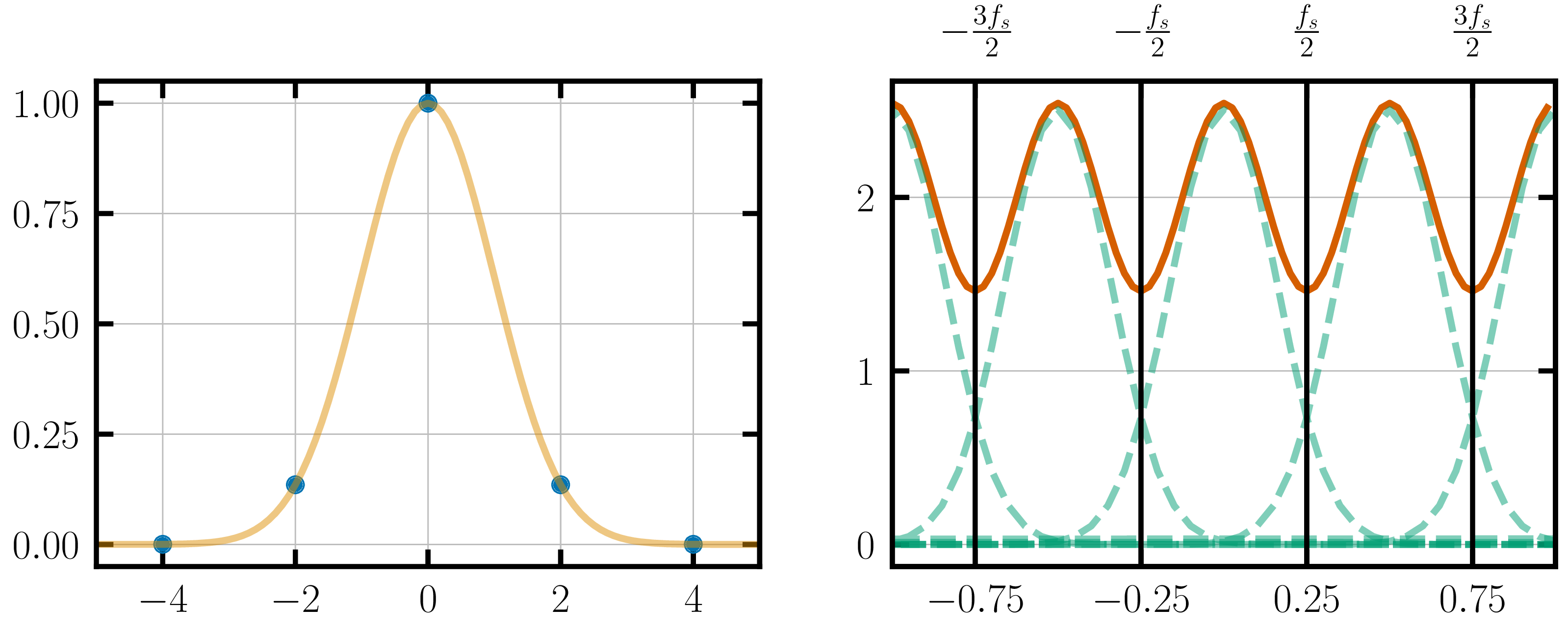
The orange line shows the discreet-time Fourier transform of the under-sampled Gaussian. The green dashed lines show copies of the FT of the original continuous Gaussian.
When analog signals are undersampled, the frequency-domain cannot capture the FT of the original signal. This is problem is called aliasing.
Aliasing can be completely eliminated for periodic functions, by sampling them at/above Nyquist frequency. For aperiodic signals that are band-limited, aliasing can be nearly eliminated by sampling them a frequency higher than the band-width. For aperiodic signals that are not band-limited, aliasing can only be mitigated by sampling at a high frequency.
A common solution to avoiding aliasing in non-bandlimited signals is to pass the analog signal through a low-pass filter that supresses the higher frequencies. Sampling the low-pass-filtered signal does not create the aliasing problem.
Nyquist Zones
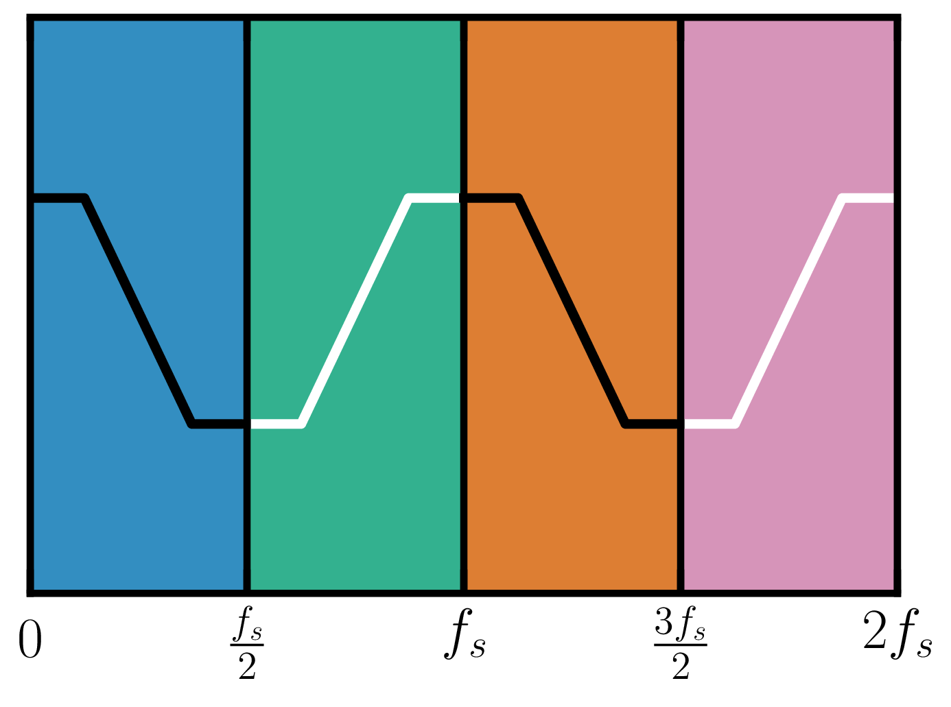
Notice that the FT of all the signals we have seen so far are either even functions or odd functions, centered around multiples of $f_s$. This is because the FT of a real and analog signal is recoverable just from the positive frequencies of the Fourier transform. Hence, the FT of a real signal sampled at $f_s$ MHz, will have all the frequency-domain information we need in each of the intervals $\left(-\frac{f_s}{2},0\right)$ MHz, $\left(0,\frac{f_s}{2}\right)$ MHz, $\left(\frac{f_s}{2},f_s\right)$ MHz, $\dots$
Each of these intervals are labelled as different Nyquist zones. In the image below, the blue region is called Nyquist Zone 1, the green region is called Nyquist Zone 2, the orange region Nyquist Zone 3 and so on.
Nyquist zones can be exploited to decrease the sampling frequency of an analog signal. Let us assume that there is an analog signal which is band-limited between 100-200 MHz. That is, the analog signal can be decomposed into sine and cosine waves that have frequencies only between 100 MHz and 200 MHz. Since the maximum frequency of the signal is 200 MHz, the sampling theorem dictates that we sample this signal at 200 MHz or higher.
However, we can exploit the knowledge that this signal does not have any frequencies in the 0-100 MHz range. Sampling this signal at 200 MHz, replicates the FT of the signal between (0,100) MHz in Nyquist Zone 1, allowing us to reconstruct the signal without loss of information.